Michael Kellett – Mym111

Power Query is the powerhouse behind Power BI’s data transformations. It’s like the kitchen where raw ingredients (data) get chopped, cleaned, and seasoned for analysis. Below, I’ve compiled ten must-know tips, divided by skill level, to help you work smarter in Power Query.

Beginner Level Tips (Getting Started with Power Query)

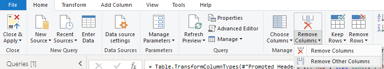
• Remove Other Columns – Keep Only What You Need, Instantly
  • Function: Remove Other Columns
  • Purpose & Result: Quickly drop all the unnecessary columns in a table except the ones you want to keep. This feature removes all columns from the table except the selected ones (learn.microsoft.com), essentially doing the reverse of deleting columns one-by-one. It’s like telling Power Query, “I only care about these columns – ditch everything else.”
  • Example: Imagine a sales data table with dozens of fields (ID codes, timestamps, etc.), but you only need Date, Product, SalesPerson, and Units for your analysis. Simply select those columns and click Remove Other Columns. Voilà – your table is trimmed to just the relevant data (no manual deleting spree needed). [Insert screenshot of using “Remove Other Columns” on a query with many columns]
  • Clarifications: This command fixes the columns that remain, which means any new columns added to the source later won’t appear in your query results unless you explicitly select them(community.fabric.microsoft.com). That’s usually a good thing – it prevents “surprise” columns from breaking your report. (Conversely, if you do want new source columns to flow in automatically, you’d use the regular Remove Columns instead(community.fabric.microsoft.com.) Overall, Remove Other Columns is a one-step way to focus your data and reduce clutter, which is especially handy when dealing with wide tables.

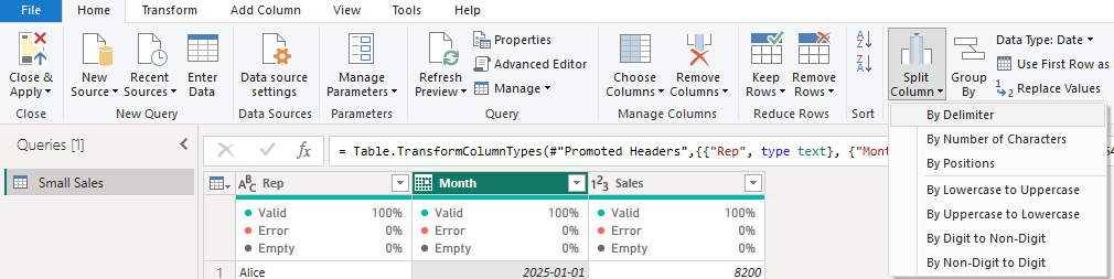
• Split Column by Delimiter – Slice and Dice Text with Ease
  • Function: Split Column (By Delimiter or Number of Characters)
  • Purpose & Result: Easily split a single text column into multiple columns (or rows) based on a delimiter or a fixed width. This helps you separate composite data – for example, splitting a full name into first and last name, or breaking an “AccountCode-Region” string into two fields. Power Query will create new columns for each part, removing the delimiter and assigning each part to its own column(radacad.com). It’s like cutting a sandwich into halves or quarters so each ingredient gets its own slice.
  • Example: Suppose you have a column FullName with values like “John Doe”. Use Split Column by Delimiter (choose space as the delimiter) to get “John” in a First Name column and “Doe” in a Last Name column. Similarly, “2019-Q4” can be split by the “-” into Year = 2019 and Quarter = Q4. [Insert screenshot of using Split Column by Delimiter on a “FullName” column]
  • Clarifications: Power Query offers splitting by common delimiters (comma, semicolon, space, etc.) or custom ones, and you can choose to split at the first delimiter, last delimiter, or each occurrence. If you have more parts than columns, PQ will create as many new columns as needed. New column names will be the original name with suffixes like “.1”, “.2”, etc., which you can rename. Also note, you can split into rows instead of columns if you want each delimited value on a new line (useful for cells containing lists)(learn.microsoft.com). Splitting is straightforward, but remember to trim any extra spaces beforehand to avoid accidental blank entries.

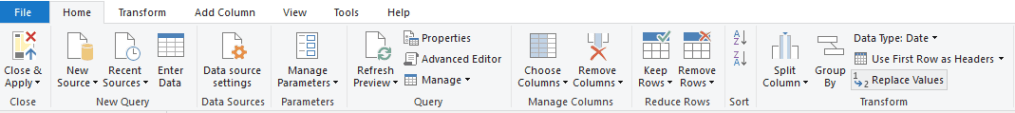
• Replace Values – Find & Fix Data Issues in One Go
  • Purpose & Result: Search for a specific value (or substring) in a column and replace it with a new value. This is your go-to for correcting typos, standardizing entries, or filling in placeholders. It works like Excel’s “find and replace,” but within your query steps – ensuring the replacements happen every time you refresh.
  • Example: Say your sales region data uses “NY” in some rows and “New York” in others, and you want consistency. You can select the Region column, choose Replace Values, and set Value to Find = “NY” and Replace With = “New York”. After clicking OK, all occurrences of “NY” in that column turn into “New York” in one step. Another example: replacing null or blank values with “N/A” or 0 for cleaner data.
  • Clarifications: By default, the replace is text-based and case-insensitive(gcomsolutions.com) – meaning “apple” will match “Apple” unless you opt to make it case-sensitive. The replacement affects the entire column, so use it carefully (it replaces every exact match of the value you specify). If you have multiple different values to swap out, you can either apply multiple Replace steps (one per value) or get fancy with a custom list replacement method. Also, ensure your column’s data type is text if you’re replacing text fragments (Power Query won’t replace part of a number, for instance, without converting it to text). Pro tip: This is great for quick data cleanup – like fixing product category names or standardizing “USA” vs “U.S.A.” – to make your subsequent analysis smoother.

Intermediate Level Tips (Taking It Up a Notch)

• Merge Queries (Joins) – Combine Tables Like a Pro
  • Purpose & Result: Merge Queries allows you to join two tables together based on a common column (think of it as a super-powered VLOOKUP that can return multiple columns)(datacamp.com). It brings in columns from one table into another, aligning rows where key values match. Use this to enrich a data table with additional info (e.g. append customer names from a lookup table onto a sales fact table by matching Customer ID).
  • Example: You have a Sales table with Product ID and a separate Products table with Product ID and Category. By merging these on Product ID, you can pull the Category into each sales row, so you can see what category each sale belongs to. In Power Query Editor, select the Sales query, click Merge Queries, choose Products as the other table, and pick Product ID in both. After the merge step is created, expand the new column to select the fields (like Category) you want to add. Now your Sales query contains the Category info for each matching Product ID. [Insert screenshot of the Merge dialog in Power Query, matching Product ID between two tables]
  • Clarifications: The default merge type is a Left Outer join – meaning all rows from the first (primary) table will remain, and matching rows from the second table are included (non-matches from the second become null). You can choose other join types (Inner, Full Outer, Anti joins, etc.) depending on your needs. Make sure the join keys have the same data type and format (no extra spaces!) to avoid missing matches. If some rows don’t find a match, you’ll see nulls – which you might need to handle (e.g., replace null with “Not Found” or similar). Merging is a game-changer for combining data from different sources, and it keeps your model tidy by letting Power Query handle the “lookup” work(geeksforgeeks.org)(geeksforgeeks.org). (Bonus tip: there’s an option for Fuzzy matching in merges – more on that in the Advanced section!)

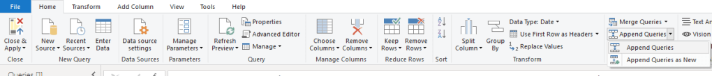
• Append Queries (Stack Data) – Union Tables for a Full Dataset
  • Purpose & Result: Appending queries stacks two or more tables on top of each other, combining them vertically into one table(geeksforgeeks.org). Use Append when you have separate datasets with the same columns (like monthly files, regional sales tables, or any similarly structured data slices) and you want to mash them into a single comprehensive table. It’s like combining pieces of the same puzzle – each table is one piece of the timeline or categories, and appending puts them all in one big table for analysis.
  • Example: Suppose you track sales in separate tables by quarter (Q1, Q2, etc.). Rather than building separate visuals for each, you can append these queries into one master SalesAllYear query. In Power Query, use Append Queries -> Append as New, and select all four quarterly queries. The result is one table with all the rows from Q1, then Q2, Q3, Q4 stacked. If Q1 had 100 rows and Q2 had 150 rows, the appended table will have 250 rows, and so on(geeksforgeeks.org). Now you can feed this consolidated data to Power BI to easily analyze the whole year. [Insert screenshot of the Append dialog selecting multiple quarterly tables]
  • Clarifications: For an append to work best, the tables should have identical column names and data types. If one table has a column the others don’t, the appended result will fill those in with nulls for the tables that lacked it(geeksforgeeks.org). Order of columns doesn’t matter (Power Query aligns by column name). A handy scenario is folder import: if you have dozens of CSVs in a folder (e.g., one per month), you can use “Folder” data source and Combine – Power Query will automatically append them and even create a custom function to import each file. After appending, consider adding a column (if needed) to mark the source (e.g., “Quarter” or “FileName”) to know where each row came from. In short, Append is your friend for aggregating data across time periods or departments into one unified table.

• Unpivot Columns – Transform a Crosstab into a Usable Table
  • Purpose & Result: Unpivoting takes data that’s laid out horizontally (multiple columns of similar values, like Jan, Feb, Mar as separate columns) and rotates it into a vertical attribute-value format(learn.microsoft.comlearn.microsoft.com). This is essential for turning “report-style” or crosstab data into a proper database-like table that Power BI can slice and dice. After unpivot, you’ll typically get two new columns: Attribute (the former column header, e.g. “Month”) and Value (the cell value under that column). It’s like taking a wide spreadsheet and turning it on its side – suddenly you have more rows but fewer columns, which is easier for analysis and filtering.
  • Example: You have a table where each row is a country and you have separate columns for Jan Sales, Feb Sales, Mar Sales. This format makes it hard to filter or chart by month. By unpivoting the month columns, you’ll get a new Month column and a single Sales column. Each country now appears in multiple rows (one per month), with “Month” = Jan, Feb, Mar, etc., and “Sales” containing the sales value. The data becomes a simple three-column table: Country, Month, Sales, which is perfect for creating a time-series visualization or performing monthly comparisons(learn.microsoft.com)(learn.microsoft.com). [Insert screenshot of a table before and after Unpivot (months across columns -> Month column with rows)]
  • Clarifications: In Power Query, you can unpivot by selecting the columns to turn into rows. Usually, it’s easiest to select the few columns you want to keep (like ID or Country) and then choose “Unpivot Other Columns” – this unpivots everything except the ones you marked to stay as-is(community.fabric.microsoft.com). The result will always produce an “Attribute” and “Value” pair by default – you’ll likely want to rename “Attribute” to something like “Month” or “Category” (whatever those former column names represent). Unpivot will remove any nulls in the unpivoted values by design (treating them as missing data). Overall, unpivoting is a lifesaver whenever you encounter that all-too-familiar “spreadsheet report” format; it lets you restructure data for meaningful analysis.

• Add Column from Examples – Let Power Query Do the Work (AI Magic!)
  • Purpose & Result: Create new columns by simply giving Power Query a few examples of the desired output, instead of manually writing a formula. This feature is like having an assistant that figures out the transformation logic for you. It’s incredibly useful when you know what result you want but aren’t sure how to get there with built-in transforms or M code. Power Query will infer the needed steps (text extraction, concatenation, date parsing, etc.) based on the examples you provide(learn.microsoft.com).
  • Example: You have separate First Name and Last Name columns and you want a single Full Name. Rather than merging columns or writing a formula, go to Add Column > Column From Examples > From All Columns. In the new example column, type the full name for the first row, e.g., “Maria Enders” (assuming Last Name = Enders, First Name = Maria). Instantly, Power Query suggests and fills the rest down the column with each person’s full name(learn.microsoft.com)(learn.microsoft.com)! It realized you wanted to concatenate First and Last Name with a space. You can do this for more complex things too, like extracting the domain from an email address or creating a category label. It’s a bit like magic – you show one example, and Power Query “reads your mind” for the rest. 🎩 [Insert screenshot of Column From Examples being used to create a Full Name column]
  • Clarifications: You can create the new column based on all existing columns or only a selection (choose “From All Columns” or “From Selection” accordingly). If the first guess isn’t correct, you can provide additional example entries in other rows to clarify the pattern. Power Query only looks at the first 100 rows to infer the logic (for performance reasons), so if your data has irregularities after that, you might need to adjust the generated formula or provide more examples covering those cases. Not all transformations are supported by examples, but many are (combining text, dates, parsing pieces of text, conditional values, etc.). After you’re satisfied, Power Query will add the column with an M formula it derived – you can always click the gear icon to see or tweak the formula. This feature is a huge time-saver, especially for those not yet comfortable with the formula language. Plus, it feels like having a little AI helper in your data prep!

Advanced Level Tips (Power Query Wizardry)

• Parameters for Dynamic Queries – Make Your Queries Flexible
  • Purpose & Result: Parameters are like variables you can use to dynamically control your query’s behavior(learn.microsoft.com)(learn.microsoft.com). You define a value once as a parameter, and reuse it in multiple places or steps – making it easy to change that value and update all related steps in one go. In practice, parameters let you do things like switch data sources (e.g., dev vs. prod database), set thresholds for filtering (e.g., a date or number cutoff), or create what-if inputs for your queries.
  • Example: Suppose you have a sales report that usually shows the last 3 months of data. You can create a parameter MonthCount = 3 and use it in your filter step (e.g., filter where Date >= Date.AddMonths(Today, -MonthCount)). Later, if you need to get 6 months of data, you just change the parameter’s value to 6 and refresh – no need to edit the filter steps themselves. Another example: a Region parameter that you use in a filter to pull data for “North America” – you could switch it to “Europe” to rerun the queries for Europe’s data. Essentially, one little parameter change can drive big query changes.
  • Clarifications: You create parameters in Power Query Editor (Home tab > Manage Parameters > New Parameter). Give it a name, data type, and a current value. Then, in your query steps, instead of a hardcoded value, you use the parameter (for instance, in a Filter Rows dialog, you can choose Parameter instead of a fixed value). Parameters are not slicers for end users; they’re mainly for the report designer’s convenience or for defining things that might change between data refreshes (though Power BI has dynamic M parameters in certain scenarios, those are a bit more advanced). Common uses include file paths, API URLs, date ranges, or any constant you might otherwise repeat in multiple queries. By using parameters, you avoid hardcoding and make your queries easier to maintain (change in one place, and all queries update). It’s a nerdy feature that brings a coding-like flexibility to your Power Query solutions – once you start using them, you’ll wonder how you managed without parameters!

• Fuzzy Matching in Merge – Join Tables Even When Keys Don’t Perfectly Match
  • Purpose & Result: Fuzzy matching allows you to merge queries even when the join keys aren’t 100% identical, by finding similar text. This is super useful in real-world data where you might have slight differences or typos in keys (e.g., “Acme Incorporated” vs “Acme Inc.”). When you enable fuzzy merge, Power Query uses algorithms (Jaccard similarity, etc.) to compare strings and match those that are likely the same, within a similarity threshold(learn.microsoft.com). The result is that you can get a “best guess” match between tables that don’t line up exactly, saving you from manually cleaning every discrepancy beforehand.
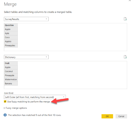
  • Example: You have a Customer table from one system and a Sales table from another. Customer names in one might include minor spelling differences compared to the other. By doing a merge on Customer Name and checking Use fuzzy matching, Power Query can match “Contoso Ltd” in one table with “Contoso Limited” in the other, or “ACME Inc” with “Acme Incorporated”. You can even get it to match nicknames (e.g., “Bob” vs “Robert”) if they’re similar enough or by providing a transformation table (a predefined map of equivalents). After merging fuzzily, you expand as usual to bring in the matched data. [Insert screenshot of Merge dialog with “Use fuzzy matching” option checked]
  • Clarifications: Fuzzy merges come with settings: Similarity Threshold (0.00 to 1.00 – higher means stricter matching; 1.00 would require exact match(learn.microsoft.com), number of matches to return, case sensitivity, etc. The default threshold is 0.8 (80% similarity). You might need to experiment with this – too low and you’ll get incorrect pairings; too high and you’ll miss true matches that have minor differences. Fuzzy matching currently works only on text columns, so ensure your keys are text. It’s also more resource-intensive than exact merges (it has to compare many combinations), so use it when needed, but try to limit the size of tables if possible (e.g., pre-filter to relevant subset before a fuzzy merge). Additionally, Power Query can return a similarity score if you enable that option, which can be useful to judge the quality of matches. In short, fuzzy merge is like a smart approximate VLOOKUP – incredibly handy for dirty data, but use with care and review the results to make sure the matches make sense for your scenario.

• Custom Functions – Reuse Your Logic (Write Once, Use Many Times)
  • Purpose & Result: A custom function in Power Query is essentially a set of steps you’ve packaged to run with different inputs. It lets you define a transformation once and reuse it easily on multiple datasets or columns(learn.microsoft.com). This is powerful for advanced scenarios, like cleaning multiple files the same way, or applying a complex operation to many columns without duplicating code. Think of it as writing your own mini Power Query tool that you can call as needed – a bit like making a recipe that you can apply to many ingredients.
  • Example: Consider you have several text columns across different tables that all require the same cleanup – say, trimming whitespace, replacing certain substrings, and making text uppercase. You can create a custom function (via Advanced Editor or the interface) called CleanText(inputText) that performs those steps on a given text value and returns the cleaned text. Then, in each query or for each column, you just invoke = CleanText([ColumnName]) in a Custom Column. Instantly, all those consistent transformations are applied everywhere. Another example: using a custom function to fetch data from a web API for a list of IDs – you write the logic once to call the API for one ID, turn it into a function, and then invoke it for each ID in a table (rather than writing the query from scratch for each).
  • Clarifications: Creating a custom function usually involves writing M code or using the “Create Function” option on an existing query. A simple way is to author a query that does what you need for one sample input, then parameterize it. For instance, you might duplicate a query and modify it to use a parameter (like a function with an argument) and then convert that query to a function. Once you have a function (it’ll appear with an fx icon in the Queries pane), you can use Invoke Custom Function to apply it. Keep in mind that custom functions execute their steps for each invocation, so be mindful of performance (applying a heavy function to thousands of rows could be slow). They can also be a bit tricky to debug, so test on a small sample first. Despite being advanced, custom functions can dramatically simplify your queries: they reduce repeated code and centralize logic. It’s like writing your own library of re-usable data prep tricks.